The Beauty and Intuition of Reinforcement Learning (Part I)

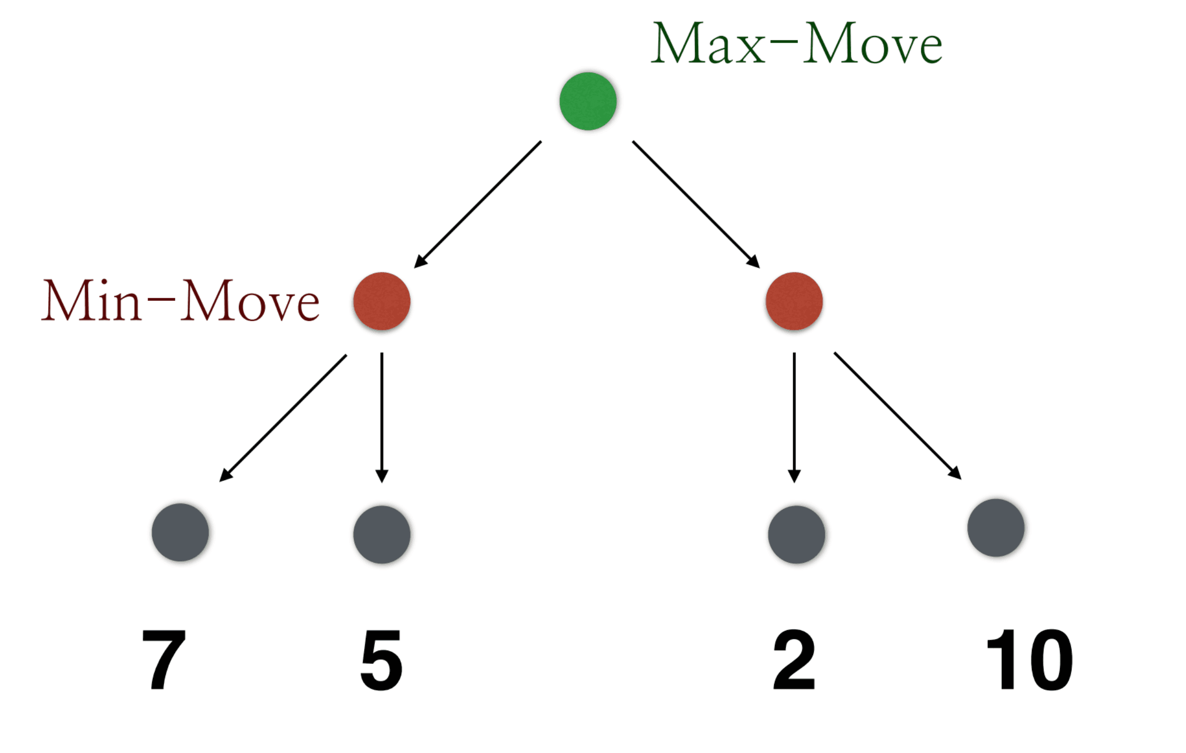
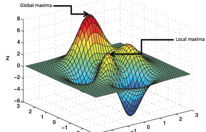
Over the past several years we've seen an explosion in the theory and applications of artificial intelligence with the rise of the transformer. It produces incredible capabilities to perform very complicated tasks like generating languages, videos, or making robots intelligent.

Yet, at its core, it's simply processing billions of tokens through intricate architectures composed of matrix multiplications streaming out another set of tokens. It might feel as if we could just tokenize the entire world, doesn't it?

Turns out the world is an exponentially large space, and in order to make sense of this complexity we need to use the right tools.

Reinforcement Learning (RL) is one such powerful tool, designed specifically for the search and discovery of solutions within vast spaces. RL doesn't exist in isolation; rather, it rests upon the foundational bedrock of classical numerical and stochastic optimization techniques, as well as connections to other rich domains, such as games.

In this series of posts, my goal is to carefully peel back the layers of this foundation, guiding you step-by-step through the evolution of search techniques. Our journey will be deliberately chronological and linear, with each topic intentionally chosen to illuminate the gradual progression toward advanced methods.

In Part I, I will cover numerical optimization techniques like Gradient Descent and Newton's Method. Part II will then motivate games as a form of search requiring the adaptability and flexibility that RL provides.

I want to thank my professor, Sicun Gao. Learning RL from multiple perspectives is difficult. I tried and failed 3 times. Never had I learned RL in such a chronological, coherent, linear way that can thread all of this content deeply together. His class was a big inspiration for writing these posts.

Throughout this journey, I'll assume you have a basic background in math and probability. If not, pull out ChatGPT and ask it questions during the read.

Numerical Optimization

Searching for the Best: The Drive to Minimize

Imagine you're looking for the best solution to a problem – perhaps the least error in a prediction, the lowest cost route on a map, or the dimmest pixel in an image. In optimization terms, "best" often means the minimum value of some objective function. We want to search through all possible inputs to discover where the output of our function is minimal. The big question is: which way do we go? How do we move through the space of possibilities to get closer to the coveted minimum?

The key lies in recognizing that our function's output changes as we adjust the input. If the output didn't change at all, there would be nothing to search for – every point would be equally good like the constant function:

But most functions do vary: some inputs give higher output, some lower. This variation is what makes search necessary—from the edge contours of a pixelated image to the clouds blending into the sky.

For a concrete analogy, think of a hiking landscape: you stand somewhere on a hilly terrain and want to find the lowest valley (minimum). The ground slopes upward in some directions and downward in others. To decide where to step, you naturally look for the direction where the ground slopes downward.

Congratulations! You've derived the first search tool called the gradient.

Level Sets and the Emergence of the Gradient

An intuitive way to see why the gradient naturally arises is by thinking in terms of level sets. A level set of a function is like a contour line on a map: it's the set of points where the function has the same value.

In a general function $f(x,y)$, a level set might be all points $(x,y)$ such that $f(x,y) = c$ for some constant $c$. If you walk along one of those contour lines in the real world, you neither gain nor lose elevation; you stay at the same height.

Now, ask yourself: if you're on the side of a hill, which direction will make you climb fastest? It's not along the contour line (that would keep you level), but straight uphill, perpendicular to the contour. So if you want to change $f$ the fastest, you have to leave the level set in the most drastic way – i.e. go orthogonal to it.

In mathematical optimization, we use this idea by looking at $-\nabla f$, the negative gradient, as the direction of steepest descent. With this insight, we're ready to use gradients as a tool for hunting the minima.

First-Order Optimization

Knowing which way is downhill is incredibly useful. First-order optimization methods are those that use the first derivative information – i.e. the gradient – to find minima. One of the most straightforward algorithms that uses gradients is the famous gradient descent (hence its name). Imagine you're blindfolded on our hilly landscape and can only sense the slope of the ground beneath your feet. Gradient descent is like taking a cautious step in the direction your feet feel the ground is sloping downward.

Then you reassess (feel the new slope at the new position) and take another step. Step by step, you move downward, always locally choosing the steepest descent direction given by the negative gradient.

It's a bit naïve in that you only look at what's happening right where you stand (you don't survey the whole landscape), but it's amazingly effective at steadily decreasing the function value. Many optimization problems, big and small, are solved exactly this way – for example, training a neural network is essentially a high-dimensional gradient descent, taking one small downhill step at a time to reduce error.

Let's derive where this "gradient descent" idea comes from in a slightly more formal way. The first-order condition for optimality is a mathematical statement of what we hinted earlier: at a local minimum (or maximum), the gradient must be zero.

If there were any slope (positive or negative) at that point, you could move a tiny bit in that direction and go lower (or higher), so it wouldn't truly be optimal. Thus, a necessary condition for $x^*$ to minimize $f(x)$ is $\nabla f(x^*) = 0$.

In reality this offers a natural stopping condition. We take itsy bitsy steps until the gradient is 0!

However, as effective as it is, gradient descent has its limitations. If the landscape is tricky – say a narrow valley where the path zigzags – the method can be slow.

Think of walking down a winding staircase: gradient descent takes the safe staircase, one step at a time.

To get to the bottom faster, we might crave a bit more information about the terrain than just "slope here, slope there." This is where we turn to the next level of understanding: second-order information.

Second-Order Insights

While first-order methods only feel the slope of the ground at your current point, second-order optimization methods also feel how the slope itself is changing. This is analogous to not just feeling the incline, but sensing whether the ground is curving or flattening out as you move.

Let's return to our landscape analogy, but now imagine you also have a special pair of glasses that let you see how curved or flat the ground is in different directions. At some points, the ground might form a curved bowl shape around you, bending upward steeply in all directions; at other points, it might form a saddle, curving up in one direction and down in another.

Why is curvature important for optimization? Because it lets us gauge whether we should accelerate or decelerate our descent in different directions. Our purple arrows in the image indicate foresighted caution: if there's strong curvature then anticipate reducing your steps. After all, "second-order" means we get a more sophisticated form of information that allows us to anticipate what's ahead. Is the valley wide and shallow? Rest assured, you can take large, stress-free steps—slope isn't going to suddenly change under your feet. Is the valley narrow and steep? I'd tread carefully.

Let's start with a simple example. To start, let's stretch this valley into a 2-dimensional space, like this

Ok, now let's move our perspective to a birds-eye-view.

Now, what are these oval-like shapes? They are the level sets! Meaning any point on a oval will evaluate to the same function value. And this makes sense. Because we know the minimum is at the center, and as we expand to outer layers, we reach function evaluations of larger values.

The intensity of the colors represent higher values of f

Now, what are these arrows? They are the sort of principal directions that represent the 2D space. For now, they seem mysterious, but only when we place a random initial point and are asked to find the minimum are we going to see the value of these directions.

The black point is our initial starting point. The gradient is the black arrow.

The green arrow—the long axis of the ellipse—tells us this direction is gentle. You can take larger steps here without overshooting.

Notice how we are not making great progress to the minimum…

That's more like it!

Now if we start at the blue arrow, we would be in a steep landscape.

This is too steep!

That's more like it!

In mathematical terms, second-order information comes from the Hessian, which is the matrix of all second partial derivatives. The Hessian matrix encodes exactly this kind of information for a multivariate function. It "describes the local curvature of a function"** in all directions around a point. In a two-dimensional case ($f(x,y)$), the Hessian is a $2\times2$ matrix involving $\frac{\partial^2 f}{\partial x^2}$, $\frac{\partial^2 f}{\partial x \partial y}$, and $\frac{\partial^2 f}{\partial y^2}$. These second derivatives tell us how quickly the slope in $x$ or $y$ changes as we move along $x$ or $y$. More intuitively, they tell us if the function is curving upward (becoming steeper uphill, like a bowl) or curving downward (like an upside-down bowl) or a mix of both (like a saddle) in each direction.

The visuals can be deceiving, but the longer the arrow means the smaller the eigenvalue. This makes sense because eigenvalues are a metric of how much the function value changes in this direction.

With curvature information, our path to the minimum can be more direct and confident, avoiding the tedious zigzagging that pure gradient descent might produce in some scenarios.

Newton's Method: Using Curvature for a Smarter Descent

The prime example of a second-order method is Newton's method for optimization. If gradient descent is like walking blindfolded, Newton's method is like a bobsled track that shoots you right to the bottom of the valley.

How does it achieve this? It builds a simple quadratic model of the function at your current point using a second-order Taylor expansion. Let's start with the one dimensional case. If you have a twice-differentiable function, you can approximate it near a point $x$ by a parabola:

This parabola (given by the first and second derivatives $f'(x)$ and $f''(x)$) is an estimate of the function's shape locally. The minimum of that parabola can be found by setting its derivative to zero: $f'(x) + f''(x),\Delta x = 0$, so the optimal step would be $\Delta x = -\frac{f'(x)}{f''(x)}$. This is the one-dimensional Newton step. It says: take the slope (first derivative) and divide by the curvature (second derivative) to decide how far to move. If the slope is large but the curvature is also very steep, you shouldn't go too far (since $f''(x)$ in the denominator is large); if the slope is large and the curvature is gentle, you can take a larger step.

In multiple dimensions, Newton's method does the analogous thing: it uses the Hessian matrix $H(x)$ (which contains all the second derivatives) to scale and rotate the step taken in the direction of the gradient. The Newton update for a multivariate function is:

Here $H^{-1} \nabla f$ plays the role of that slope-over-curvature division from one dimension (with the matrix inverse generalizing the division). What this means is Newton's method looks at the local bowl-shaped approximation of $f$ at $x_{current}$ and jumps directly to the bottom of that bowl. If the function really were a perfect quadratic bowl, Newton's step would land you exactly at the minimum in one shot.

It's important to mention that Newton's method, for all its speed and elegance, isn't without caveats. Computing the Hessian for complex problems can be expensive, and if the function's Hessian is not positive-definite (e.g. at a saddle point or maximum), the method can misbehave. There are modifications and precautions to handle these issues (like adding damping or using quasi-Newton methods that approximate the Hessian). But conceptually, Newton's method shines as the pinnacle of using local information: it combines first-order slope and second-order curvature to navigate the space of solutions as efficiently as possible.

Wrapping up Numerical Optimization

We've looked at only a few examples of how gradient-based information helps us navigate the minimization problem. However, amidst even the individual algorithmic shortcomings in Newton's method and the like, we've only solved part of the puzzle. For one, these techniques assume global solutions for only convex functions. If this assumption was removed, we'd only be guaranteed local minima solutions. If we start in a local valley, how can we look past that?

Also, we have made big assumptions on the function itself—specifically that it is continuously differentiable and smooth. Without these guarantees, we could be dealing with some crazy functions, in which other methods are better suited (like the stupidly simple three-point method).

Stochastic Search

In numerical optimization so far, we mainly used local search methods (like gradient descent) that greedily follow the slope to find a nearby minimum. This works well when the problem has a nice unimodal shape or when we only need a local minimum. However, many real landscapes are rugged with exponentially many local minima. To find the true global optimum, you might need to climb out of a smaller valley and explore other regions. In optimization, this means introducing randomness into the search. By occasionally allowing moves that don't immediately improve the objective, we give the algorithm a chance to explore. Randomness provides a way to escape local traps and search the whole landscape for a better solution.

Cross-Entropy Method (CEM)

The Cross-Entropy Method (CEM) takes randomness by working with a whole distribution of solutions at once.

Ok back to CEM. Instead of having one hiker exploring the landscape, imagine we release a swarm of explorers or sample many random points across the terrain.

With CEM, we maintain a probability distribution over the solution space and iteratively update this distribution to focus in on the best regions. Although we can use any distribution, we will use Gaussians for it's simplicity and intuitive parameters. Gaussians contain two parameters: the mean $\mu$ and covariance $\Sigma$.

You can think of $\mu$ almost like the lead hiker. He knows the terrain the best because he sits in the center of all the hikers, who feed information to him at the top. He can allow any hiker to explore any area within a certain radius defined by $\Sigma$. And as a lost wanderer, you may stumble upon any of the hikers and sample their location (in red).

We don't rely on local gradient information at all; CEM is a derivative-free global optimizer. This means it can handle "black-box" functions where gradients are unavailable or the landscape is extremely rugged. This helps us with our conundrum back in the Numerical Optimization section.

CEM repeatedly performs two phases – sampling and updating.

We also choose a fraction of "elite" samples to guide the update. Here's a basic outline of the CEM algorithm

• 1. Sample a population: Draw $N$ random candidate solutions from the current probability distribution. Evaluate each candidate's objective function value.
• 2. Select elites: Rank the $N$ samples by performance (say we are minimizing the cost, so rank from lowest cost to highest). Take the top $M$ samples (the best $M$, where $M = \rho N$ for some chosen elite proportion $\rho$, e.g. $\rho=0.2$ for the top 20%) as the elite set. These are like the fittest individuals in an evolutionary sense – the ones with highest performance.
• 3. Update the distribution: Adjust the parameters of the sampling distribution to get closer to these elite samples. Concretely, we use the elite set to compute a new mean and covariance for the Gaussian. In fact, this step can be seen as finding the maximum likelihood estimate of the distribution given the elite data. For a Gaussian, the new mean might be the average of the elite solutions, and the new covariance reflects how spread-out or concentrated those elite solutions are in each direction.
• 4. Repeat: Using the updated distribution, go back to step 1 and generate a new batch of samples, iteratively refining the search distribution. Stop when the distribution converges (e.g. very small covariance, meaning it has focused on a narrow region) or after a fixed number of iterations.

This procedure gradually focuses the search. Over iterations, the distribution "homes in" on what looks like the best part of the landscape.

CEM's distribution-driven approach is powerful because it learns the shape of the search space from samples. We are not following gradients at a point, but rather using statistics of many points to infer where to search next.

Search Gradient

Up to now, we have been optimizing the original function $f(x)$ directly with respect to $x$. This meant we were deterministically evaluating the function at specific points x to inform our direction within the domain..Instead, why don't we optimize the parameters of a probability distribution that generates candidate $x$'s?

As we've discussed earlier, deterministic methods limited you to evaluating only $f(x)$ itself, meaning you could only take small, cautious steps around $x$ to carefully sense your direction. But with a search gradient, we gain the freedom to sample many points within the domain simultaneously.

Remember this because it's very important: probabilities give us flexibility. We can now elegantly express the quantity we aim to minimize as an expectation:

Don't panic—let's take a moment to digest this. Essentially, all we've introduced is the expectation operator, symbolized by "E". Practically, we can approximate this expectation by simply computing a sample mean using Monte Carlo sampling (we'll explore this further soon):

In other words, this expected value is essentially just a weighted sum of two fundamental components multiplied together:

1. The function evaluations themselves, $f(x)$, exactly what we had before
2. The probability associated with each function evaluation.

Recall that $f(x)$ provides a pure, focused signal indicating exactly what we're minimizing. The introduction of probabilities, however, complicates matters slightly: it diffuses this clean signal across numerous other points, including those potentially worse than our current choice!

While this pessimistic mindset is totally reasonable, we can also think optimistically. Think of the probabilities are there to be more optimistic and explorative—to never prematurely settle on a candidate unless we're truly confident it's an excellent minimum. It's akin to an indecisive child hesitant to choose just one flavor of ice cream, always holding out for a better option.

How do we start? The only static pieces of information that help guide us to the optimum are the parameters like the mean and covariance, so let's define some randomly initialized values for them.

With these initialized parameters, we can start to sample from them! Below are a few iterations side by side

1. Sample candidate solutions $x_i$ from the current distribution:

   $$x_i \sim p\left(x ; \theta_t\right), \quad i=1,2, \ldots, N$$

2. Evaluate $f\left(x_i\right)$ for each candidate solution $x_i$.

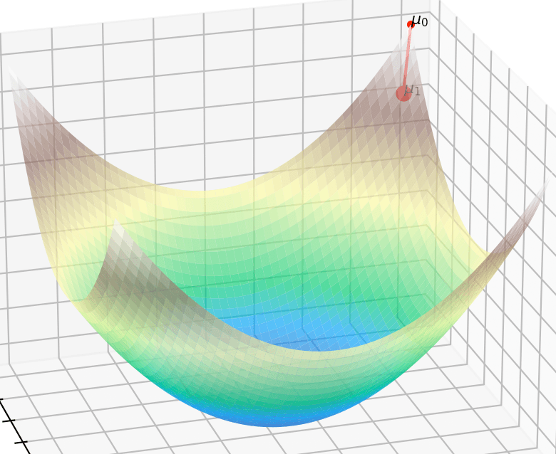
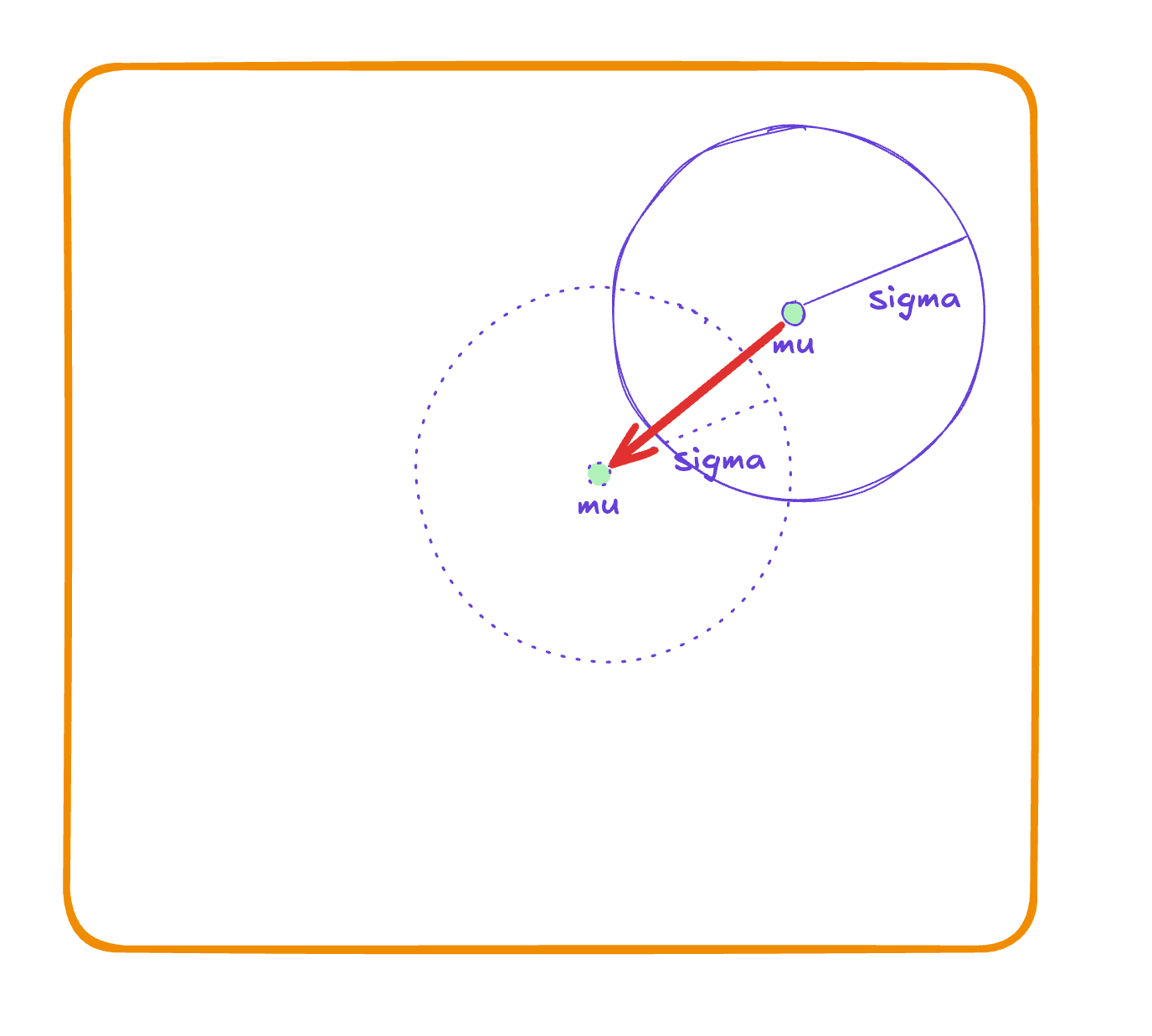
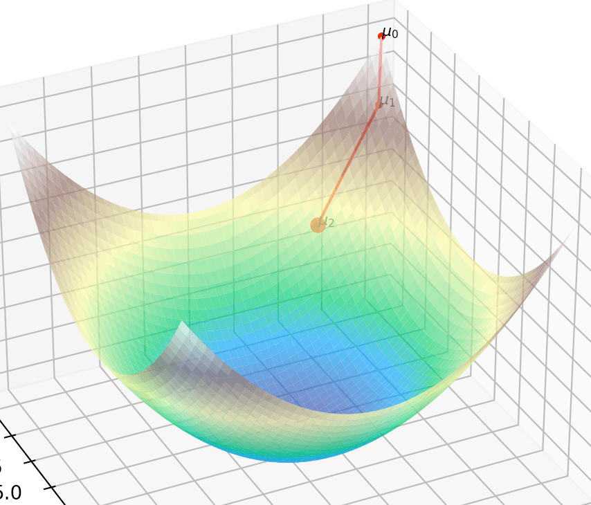
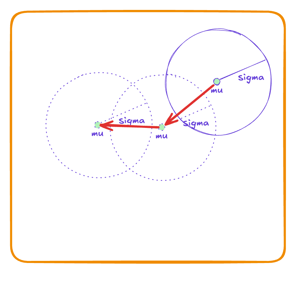
3. Evaluate the log probability

What we have done with Gradient Descent, we chose the direction of maximum descent, which meant going in the orthogonal direction of the level set. But this time, we take the gradient with respect to theta, our distribution parameters! So it's like we're sliding down a different landscape. We therefore add another symbol that represents this gradient, $\nabla_\theta$:

Ok let's move the gradient symbol inside the expectation:

Ok don't panic, but now we have to compute something particularly nasty. We do something called the "log trick" for mathematical reasons (If more curious ask an LLM!). But this will turn out to be a very nice property when we use it later.

Ok! We finally have the direction we can go in our parameterized space. Now we can take the update, just like we did in GD:

Intuitively speaking, we can interpret the magnitude of our update direction as a balancing act: it robustly nudges the distribution's parameters toward regions of higher probability in the $\theta$-space. Within those promising regions, we naturally take smaller, more cautious steps when $f(x)$ is low, ensuring we remain close to good solutions. Conversely, larger values of $f(x)$ propel us away more aggressively, steering us clear of poorer regions.

Conclusion

Through engaging analogies and mathematical insight, we built intuition for these stochastic search methods. Randomness is the thread that ties them together: it allows exploring the unknown and avoidance of local optima. In the next section, we are going to use this tool of randomness to construct higher abstract landscapes, often through the lens of games.

Acknowledgements

I'd like to thank friends who have proofread my writing and contributed essential feedback to make this work happen: Ryan Lavin.